![]()
Python Big Data Platform
Brief Overview and Introduction
General Aspects and Trials
The Python Quant Platform is developed and maintained by The Python Quants GmbH. It offers Web-/browser-based data and financial analytics for individuals, teams and organizations. Free registrations are possible under http://trial.quant-platform.com.
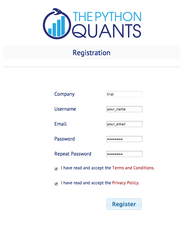
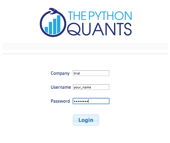
You can freely choose your your_user_name and password. You can then login under http://analytics.quant-platform.com, using trial as company in combination with your_user_name and password.
Please note that trial/test accounts are only for illustration purposes and they can be closed at any time (with all data, code, etc. be permanently deleted).
Please read also the Terms & Conditions as well as our Privacy Policy.
If you have questions about the platform or any troubles, you can reach us under platform@pythonquants.com.
Platform Components & Features
At the moment, the Python Quant Platform comprises the following components and features:
- IPython Notebook: interactive data and financial analytics in the browser with full Python integration and much more (cf. IPython home page).
- Anaconda Python Distribution: complete Python stack for financial, scientific and data analytics workflows/applications (cf. Anaconda page); you can easily switch between Python 2.7 and 3.4.
- R Stack: for statistical analyses, integrated via
rpy2and IPython Notebook - DX Analytics: our library for advanced financial and derivatives analytics with Python based on Monte Carlo simulation.
- File Manager: a GUI-based File Manager to upload, download, copy, remove, rename files on the platform.
- Chat/Forum: there is a simple chat/forum application available via which you can share thoughts, documents and more.
- Collaboration: the platform features user/group administration as well as file sharing via public folders.
- Linux Server: the platform is powered by Linux servers to which you have full shell access.
- Deployment: the platform is easily scalable since it is cloud-based and can also be easily deployed on your own servers (via Docker containers).
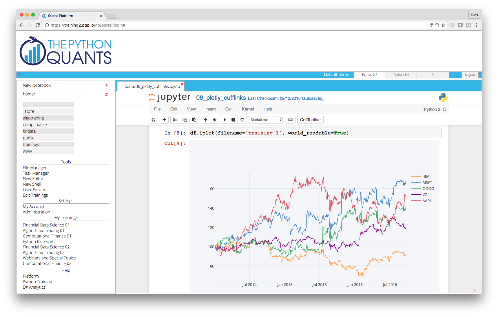
IPython Notebook
In the left panel of the platform, you find the current working path indicated (in black) as well as the current folder and file structure (as links in purple). Note that in this panel only IPython Notebook files are displayed. Here you can navigate the current folder structure by clicking on a link. Clicking on the double points ".." brings you one level up in the structure. Clicking the refresh button right next to the double points updates the folder/file structure. Clicking on a file link opens the IPython Notebook file.
Basic Approach
You find a link to open a new notebook on top of the left panel. With IPython notebooks, like with this one, you can interactively code Python and do data/financial analytics.
print ("Hello Quant World.")
# simple calculations
3 + 4 * 2
# working with NumPy arrays
import numpy as np
rn = np.random.standard_normal(100)
rn[:10]
# plotting
import matplotlib.pyplot as plt
%matplotlib inline
plt.plot(rn.cumsum())
plt.grid(True)

IPython Notebook as a system shell.
!ls -n
!mkdir test
!ls
!rm -r test
IPython Notebook as a media integrator. Here a talk by Yves about "Interactive Analytics of Large Financial Data Sets" with Python & IPython.
from IPython.display import YouTubeVideo
YouTubeVideo(id="XyqlduIcc2g", width=700, height=400)
Efficient Financial Analytics
Combining the pandas library with IPython Notebook makes for a powerful financial analytics environment.
import pandas as pd
import pandas.io.data as web
AAPL = web.DataReader('AAPL', data_source='google')
  # reads data from Google Finance
AAPL['42d'] = pd.rolling_mean(AAPL['Close'], 42)
AAPL['252d'] = pd.rolling_mean(AAPL['Close'], 252)
  # 42d and 252d trends
AAPL[['Close', '42d', '252d']].plot(figsize=(10, 5))

DX Analytics
DX Analytics is a Python library for advanced financial and derivatives analytics written by The Python Quants. It is particularly suited to model multi-risk derivatives and to do a consistent valuation of portfolios of complex derivatives. It mainly uses Monte Carlo simulation since it is the only numerical method capable of valuing and risk managing complex, multi-risk derivatives books.
An example with an European maximum call option on two underlyings.
import dx
%run dx_example.py
  # sets up market environments
  # and defines derivative instrument
max_call.payoff_func
  # payoff of a maximum call option
  # on two underlyings (European exercise)
max_call.vega('jd')
  # numerical Vega with respect
  # to one risk factor
We are going to generate a Vega surface for one risk factor with respect to the initial values of both risk factors.
asset_1 = np.arange(28., 46.1, 2.)
asset_2 = asset_1
a_1, a_2 = np.meshgrid(asset_1, asset_2)
value = np.zeros_like(a_1)
%%time
vega_gbm = np.zeros_like(a_1)
for i in range(np.shape(vega_gbm)[0]):
    for j in range(np.shape(vega_gbm)[1]):
        max_call.update('gbm', initial_value=a_1[i, j])
        max_call.update('jd', initial_value=a_2[i, j])
        vega_gbm[i, j] = max_call.vega('gbm')
dx.plot_greeks_3d([a_1, a_2, vega_gbm], ['gbm', 'jd', 'vega gbm'])
  # Vega surface plot

Parallel Processing
Monte Carlo simulation is a computationally demanding task that nowadays in the financial industry is implemented generally on a large scale (eg for Value-at-Risk or Credit-Value-Adjustment calculations).
import math
This function simulates a geometric Brownian motion.
def simulate_geometric_brownian_motion(p):
    M, I = p
      # time steps, paths
    S0 = 100; r = 0.05; sigma = 0.2; T = 1.0
      # model parameters
    dt = T / M
    paths = np.zeros((M + 1, I))
    paths[0] = S0
    for t in range(1, M + 1):
        paths[t] = paths[t - 1] * np.exp((r - 0.5 * sigma ** 2) * dt +
                    sigma * math.sqrt(dt) * np.random.standard_normal(I))
    return paths
An example simulation with the function.
%time paths = simulate_geometric_brownian_motion((50, 100000))
  # example simulation
plt.plot(paths[:, :10]); plt.grid()

Now using the multiprocessing module of Python.
from time import time
import multiprocessing as mp
I = 7500  # number of paths
M = 50  # number of time steps
t = 100 # number of tasks/simulations
# running with a max of 8 cores
times = []
for w in range(1, 9):
    t0 = time()
    pool = mp.Pool(processes=w)
    result = pool.map(simulate_geometric_brownian_motion, t * [(M, I), ])
    times.append(time() - t0)
And the performance results visualized.
plt.plot(range(1, 9), times)
plt.plot(range(1, 9), times, 'ro')
plt.grid(True)
plt.xlabel('number of threads')
plt.ylabel('time in seconds')
plt.title('%d Monte Carlo simulations' % t)

Statistics with R
We analyze the statistical correlation between the EURO STOXX 50 stock index and the VSTOXX volatility index.
First the EURO STOXX 50 data.
import pandas as pd
cols = ['Date', 'SX5P', 'SX5E', 'SXXP', 'SXXE',
        'SXXF', 'SXXA', 'DK5F', 'DKXF', 'DEL']
es_url = 'http://www.stoxx.com/download/historical_values/hbrbcpe.txt'
try:
    es = pd.read_csv(es_url,  # filename
                     header=None,  # ignore column names
                     index_col=0,  # index column (dates)
                     parse_dates=True,  # parse these dates
                     dayfirst=True,  # format of dates
                     skiprows=4,  # ignore these rows
                     sep=';',  # data separator
                     names=cols)  # use these column names

    # deleting the helper column
    del es['DEL']
except:
    # read stored data if there is no Internet connection
    es = pd.HDFStore('data/SX5E.h5', 'r')['SX5E']
Second, the VSTOXX data.
vs_url = 'http://www.stoxx.com/download/historical_values/h_vstoxx.txt'

try:
    vs = pd.read_csv(vs_url,  # filename
                     index_col=0,  # index column (dates)
                     parse_dates=True,  # parse date information
                     dayfirst=True, # day before month
                     header=2)  # header/column names
except:
    # read stored data if there is no Internet connection
    vs = pd.HDFStore('data/V2TX.h5', 'r')['V2TX']
Bridging to R from within IPython Notebook and pushing Python data to the R run-time.
%load_ext rpy2.ipython
import numpy as np
# log returns for the major indices' time series data
datv = pd.DataFrame({'SX5E' : es['SX5E'], 'V2TX': vs['V2TX']}).dropna()
rets = np.log(datv / datv.shift(1)).dropna()
ES = rets['SX5E'].values
VS = rets['V2TX'].values
%Rpush ES VS
Plotting with R in IPython Notebook.
%R plot(ES, VS, pch=19, col='blue'); grid(); title("Log returns ES50 & VSTOXX")

Linear regression with R.
%R c = coef(lm(VS~ES))
%R plot(ES, VS, pch=19, col='blue'); grid(); abline(c, col='red', lwd=5)

Pulling data from R to Python
%Rpull c
import matplotlib.pyplot as plt
%matplotlib inline
plt.figure(figsize=(9, 6))
plt.plot(ES, VS, 'b.')
plt.plot(ES, c[0] + c[1] * ES, 'r', lw=3)
plt.grid(); plt.xlabel('ES'); plt.ylabel('VS')

Bayesian Statistics
The example we use is a "classical" pair traiding strategy, namely with gold and stocks of gold mining companies both represented by ETFs with symbols
GLD(GLD background) andGDX(GDX background), respectively.
Example courtesy of Thomas Wiecki (@twiecki).
We use zipline and PyMC3 for the analysis.
import numpy as np
import pymc as pm
import zipline
import pytz
import datetime as dt
First, we load the data from the Web.
try:
    datg = zipline.data.load_from_yahoo(stocks=['GLD', 'GDX'],
             end=dt.datetime(2014, 3, 15, 0, 0, 0, 0, pytz.utc)).dropna()
except:
    datg = pd.HDFStore('data/gold.h5', 'r')['datg']
%matplotlib inline
datg.plot(figsize=(9, 5))

A scatter plot of the value pairs over time and a simple linear regression.
import matplotlib as mpl; import matplotlib.pyplot as plt
mpl_dates = mpl.dates.date2num(data.index)
plt.figure(figsize=(9, 5))
plt.scatter(datg['GDX'], datg['GLD'], c=mpl_dates, marker='o')
reg = np.polyfit(datg['GDX'], datg['GLD'], 1)
plt.plot(datg['GDX'], np.polyval(reg, datg['GDX']), 'r-', lw=3)
plt.grid(True); plt.xlabel('GDX'); plt.ylabel('GLD')
plt.colorbar(ticks=mpl.dates.DayLocator(interval=250),
             format=mpl.dates.DateFormatter('%d %b %y'))

We implement a Bayesian random walk model (I).
model_randomwalk = pm.Model()
with model_randomwalk:
    sigma_alpha, log_sigma_alpha = \
            model_randomwalk.TransformedVar('sigma_alpha',
                            pm.Exponential.dist(1. / .02, testval=.1),
                            pm.logtransform)
    sigma_beta, log_sigma_beta = \
            model_randomwalk.TransformedVar('sigma_beta',
                            pm.Exponential.dist(1. / .02, testval=.1),
                            pm.logtransform)
We implement a Bayesian random walk model (II).
from pymc.distributions.timeseries import GaussianRandomWalk

# take samples of 50 elements each
subsample_alpha = 50
subsample_beta = 50

with model_randomwalk:
    alpha = GaussianRandomWalk('alpha', sigma_alpha**-2,
                               shape=len(datg) / subsample_alpha)
    beta = GaussianRandomWalk('beta', sigma_beta**-2,
                              shape=len(datg) / subsample_beta)

    alpha_r = np.repeat(alpha, subsample_alpha)
    beta_r = np.repeat(beta, subsample_beta)
We implement a Bayesian random walk model (III).
with model_randomwalk:
    # define regression
    regression = alpha_r + beta_r * datg.GDX.values[:1950]

    sd = pm.Uniform('sd', 0, 20)
    likelihood = pm.Normal('GLD', mu=regression,
                sd=sd, observed=datg.GLD.values[:1950])
We implement a Bayesian random walk model (IV).
import warnings; warnings.simplefilter('ignore')
import scipy.optimize as sco
with model_randomwalk:
    # first optimize random walk
    start = pm.find_MAP(vars=[alpha, beta], fmin=sco.fmin_l_bfgs_b)

    # sampling
    step = pm.NUTS(scaling=start)
    trace_rw = pm.sample(100, step, start=start, progressbar=False)
The plot of the regression coefficients over time.
part_dates = np.linspace(min(mpl_dates), max(mpl_dates), 39)
fig, ax1 = plt.subplots(figsize=(10, 5))
plt.plot(part_dates, np.mean(trace_rw['alpha'], axis=0),
         'b', lw=2.5, label='alpha')
for i in range(45, 55):
    plt.plot(part_dates, trace_rw['alpha'][i], 'b-.', lw=0.75)
plt.xlabel('date'); plt.ylabel('alpha'); plt.axis('tight')
plt.grid(True); plt.legend(loc=2)
ax1.xaxis.set_major_formatter(mpl.dates.DateFormatter('%d %b %y') )
ax2 = ax1.twinx()
plt.plot(part_dates, np.mean(trace_rw['beta'], axis=0),
         'r', lw=2.5, label='beta')
for i in range(45, 55):
    plt.plot(part_dates, trace_rw['beta'][i], 'r-.', lw=0.75)
plt.ylabel('beta'); plt.legend(loc=4); fig.autofmt_xdate()

The plot of the regression lines over time.
plt.figure(figsize=(10, 5))
plt.scatter(datg['GDX'], datg['GLD'], c=mpl_dates, marker='o')
plt.colorbar(ticks=mpl.dates.DayLocator(interval=250),
             format=mpl.dates.DateFormatter('%d %b %y'))
plt.grid(True); plt.xlabel('GDX'); plt.ylabel('GLD')
x = np.linspace(min(datg['GDX']), max(datg['GDX']))
for i in range(39):
    alpha_rw = np.mean(trace_rw['alpha'].T[i])
    beta_rw = np.mean(trace_rw['beta'].T[i])
    plt.plot(x, alpha_rw + beta_rw * x, color=plt.cm.jet(256 * i / 39))

Vector Auto Regression
Let us apply Multi-Variate Auto Regression to the financial time series data we have:
- GLD
- GDX
- EURO STOXX 50
- VSTOXX
Let us resample and join the data sets.
datv.index = datv.index.tz_localize(pytz.utc)
datf = datg.join(datv, how='left')
datf = datf.resample('1M', how='last')
  # resampling to monthly data
# datf = datf / datf.ix[0] * 100
  # uncomment for normalized starting values
# datf = np.log(datf / datf.shift(1)).dropna()
  # uncomment for log return based analysis
The starting values of the time series data we use.
datf.head()
We use the VAR class of the statsmodels library.
from statsmodels.tsa.api import VAR
model = VAR(datf)
lags = 5
  # number of lags used for fitting
results = model.fit(maxlags=lags, ic='bic')
  # model fitted to data
The summary statistics of the model fit.
results.summary()
Historical data and forecasts.
results.plot_forecast(50, figsize=(8, 8), offset='M')
  # historical/input data and
  # forecasts given model fit

Integrated simulation of the future development of the financial instrument prices/levels.
results.plotsim(paths=5, steps=50, prior=False,
                initial_values=datf.ix[-1].values,
                figsize=(8, 12), offset='M')
  # simulated paths given fitted model

File Manager
The File Manager allows the easy, GUI-based file management on the platform.
Left Column
In the left column you can navigate the file system. For instance, you find a folder called public which you can use to share files with others.
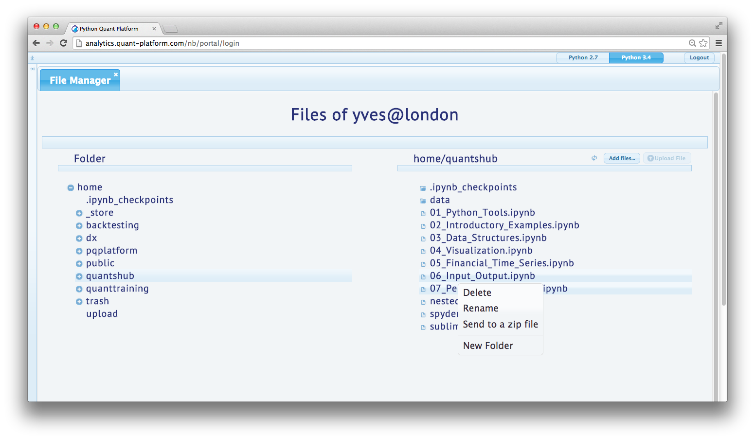
Right Column
In the right column, you find the contents of the folder currently active in the left column. The content is updated by clicking on the refresh butotn. You can, for example, drag and drop files and folders as well as upload files from you local disk. For uploading, you have to do the following:
- press the add files button
- select (multiple) file(s) from your local disk
- press the upload button
Via a double click on a file, you can download it.
In addition, via a right click on a file, you can:
- delete a file/folder
- rename a file/folder
- zip a file/folder
- generate a new folder
All file operations are only implementable based on the respective user's rights on the operating system level. For example, everybody can copy a file to the public folder. This file can then be read and executed by everybody, but only the "owner" of the file can overwrite or delete it.
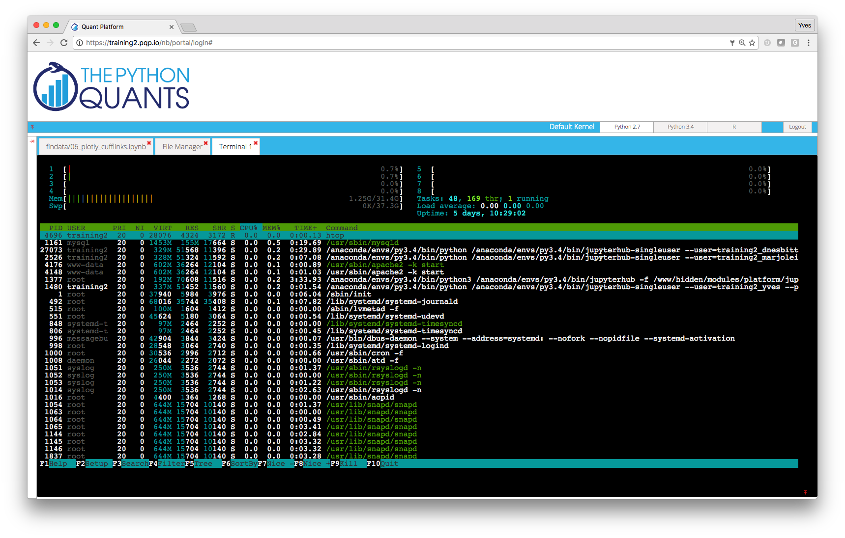
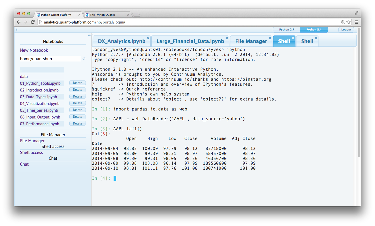
Shell Access
This component of the platform allows the shell-based access to the Linux server. This part of the platform requires a separate login for security reasons (credentials available upon request).
IPython Shell
For example, you can also interactively code on the shell via IPython Shell. The IPython Shell version is started by simply typing ipython in the system shell.
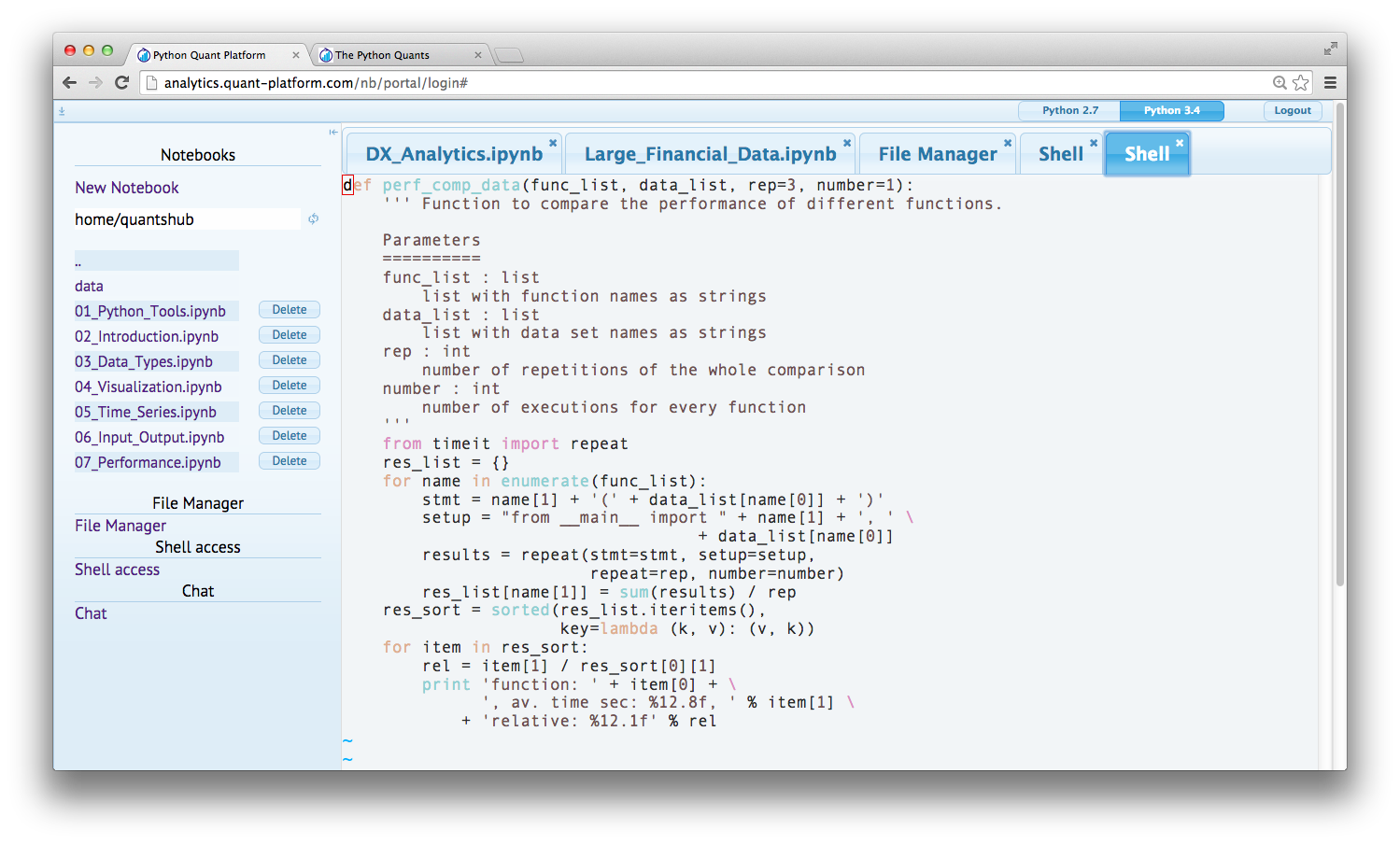
Text Editing and Coding
Via the system shell you can of course edit and kind of text document and file with computer code, e.g. Python. To this end, you can use Vim which is started via typing vim filename on the system shell or alternatively Nano (started by nano filename).
File Operations and Git Repositories
Of course, you can do anything else via the system shell given your personal rights on the operating system level. Among others, you can:
- do file operations (copying, renaming, moving, etc.)
- use Git repositories (to clone/pull projects, commit and push them)
Deployment Scenarios & Use Cases
- Getting Started with Python at high school, university, trainings, corporations, institutions, etc.
- Browser-based Data Analytics at universities, companies, financial institutions, etc.
- Browser-based Financial Analytics based on interactive exploration, (automated) workflows, applications
- Browser-based Usage of Infrastructure for desktops, servers, grid, cloud, etc.
- Browser-based Python Development for all kinds of Python projects
Technically, the platform can be deployed in almost any Linux-based hardware environment:
- dedicated server like the trial server (8 Cores, 16 GB Ram)
- cloud instances like a Digital Ocean droplet (from the smallest one with 1 Core, 512MB)
- hosted and on premise behind your firewalls
Deployment with and without Docker container usage. White labeling easily possible.
Recent, selected use cases of the platform.
- Provision of IPython Notebooks from "Python for Finance" (O'Reilly) book
- Use during NumPy + pandas Training for NYC-based Hedge Fund
- Use during Python for Quant Finance Training in London
- Hosting of IPython Notebooks for German financial institution
- Interactive Collaboration with South African client during Python project
Consulting and Development Services
The Python Quants group – i.e. The Python Quants GmbH, Germany, and The Python Quants LLC., New York City – provide consulting and development services with a focus on Python for Finance. The team consists of Python and Financial experts with comprehensive experience in the financial industry and in particular in the Quant Finance space.
For example, The Python Quants have designed and implemented a Python-based Tutorial for Eurex, one of the leading derivatives exchanges in the world. The tutorial is about volatility derivatives and is called VSTOXX Advanced Services and is available under http://www.eurexchange.com/vstoxx/. There are is also strategy backtesting application available under http://www.eurexchange.com/vstoxx/app2/
Python for Quant Finance Trainings
The Python Quants group offers trainings on a global basis. Training offerings include, among others:
- Python for Finance
- Derivatives Analytics with Python
- Performance Python
During trainings, the Python Quant Platform is used for a frictionless start and a highly interactive, collaborative training experience.
There is also a complete Python for Finance Online Course available under http://quantshub.com.
from IPython.display import HTML
HTML('<iframe src=http://quantshub.com/content/python-finance-yves-j-hilpisch width=90% height=500></iframe>')
Python for Quant Finance Books
There are two books available from The Python Quants group about Python for Quant Finance.
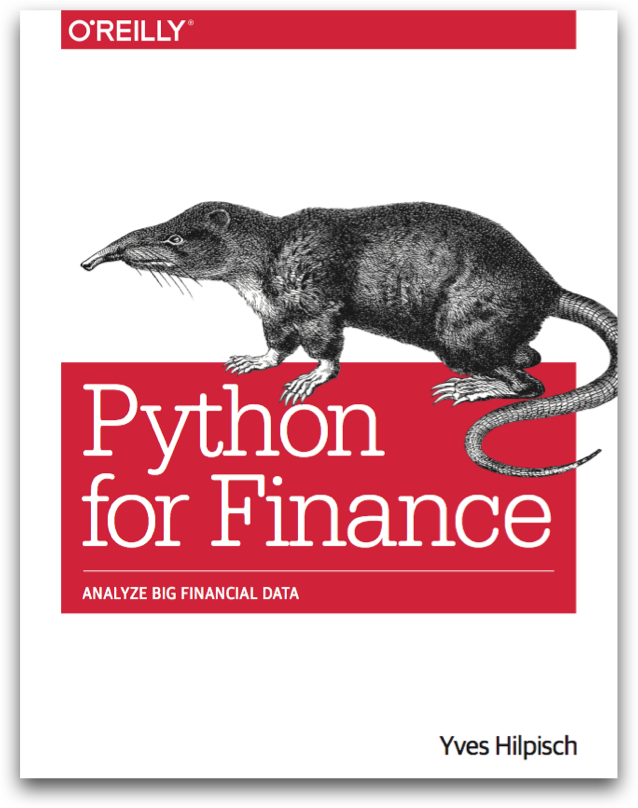
Python for Finance
Derivatives Analytics with Python
The other book by The Python Quants group is about advanced, market-based derivatives analytics and uses Python to illustrate and implement all numerical methods introduced (Fourier-based option pricing, Monte Carlo simulation, option model calibration, hedging).
The book will be published in 2015 by Wiley Finance. See http://derivatives-analytics-with-python.com.
Community and Conferences
Members of The Python Quant group are actively involved in the Python community and organize different meetup groups both in Europe as well as in New York City:
The Python Quants also organize the largest "For Python Quants" conference in the world. At the recent NYC conference in March 2014, more than 220 people have been in attendance (cf. http://forpythonquants.com). The next one will take place in London on 28. November 2014.
Contact us
Please contact us if you have any questions or want to get involved in our Python community events.
![]()
Python Quant Platform | http://quant-platform.com
Derivatives Analytics with Python | Derivatives Analytics @ Wiley Finance
Python for Finance | Python for Finance @ O'Reilly