![]()
Python – A Solution to "Big" Data Problems?
Dr. Yves J. Hilpisch
The Python Quants GmbH
Universidad Politécnica de Madrid – 12. February 2014
About Me
A brief bio:
- Managing Partner of The Python Quants
- Founder of Visixion GmbH – The Python Quants
- Lecturer Mathematical Finance at Saarland University
- Focus on Financial Industry and Financial Analytics
- Book (2013) "Derivatives Analytics with Python"
- Book (July 2014) "Python for Finance", O'Reilly
- Dr.rer.pol in Mathematical Finance
- Graduate in Business Administration
- Martial Arts Practitioner and Fan
See www.hilpisch.com
Python for Analytics
Corporations, decision makers and analysts nowadays generally face a number of problems with data:
- sources: data typically comes from different sources, like from the Web, from in-house databases or it is generated in-memory, e.g. for simulation purposes
- formats: data is generally available in different formats, like SQL databases/tables, Excel files, CSV files, arrays, proprietary formats
- structure: data typically comes differently structured, be it unstructured, simply indexed, hierarchically indexed, in table form, in matrix form, in multidimensional arrays
- completeness: real-world data is generally incomplete, i.e. there is missing data (e.g. along an index) or multiple series of data cannot be aligned correctly (e.g. two time series with different time indexes)
- conventions: for some types of data there a many “competing” conventions with regard to formatting, like for dates and time
- interpretation: some data sets contain information that can be easily and intelligently interpreted, like a time index, others not, like texts
- performance: reading, streamlining, aligning, analyzing – i.e. processing – (big) data sets might be slow
In addition to these data-oriented problems, there typically are organizational issues that have to be considered:
- departments: the majority of companies is organized in departments with different technologies, databases, etc., leading to “data silos”
- analytics skills: analytical and business skills in general are possessed by people working in line functions (e.g. production) or administrative functions (e.g. finance)
- technical skills: technical skills, like retrieving data from databases and visualizing them, are generally possessed by people in technology functions (e.g. development, systems operations)
This presentation focuses on
- Python as a general purpose data analytics environment
- interactive analytics examples
- prototyping-like Python usage
It does not address such important issues like
- architectural issues regarding hardware and software
- development processes, testing, documentation and production
- real world problem modeling
Some Python Fundamentals
Fundamental Python Libraries
A fundamental Python stack for interactive data analytics and visualization should at least contain the following libraries tools:
- Python – the Python interpreter itself
- NumPy – high performance, flexible array structures and operations
- SciPy – collection of scientific modules and functions (e.g. for regression, optimization, integration)
- pandas – time series and panel data analysis and I/O
- PyTables – hierarchical, high performance database (e.g. for out-of-memory analytics)
- matplotlib – 2d and 3d visualization
- IPython – interactive data analytics, visualization, publishing
It is best to use either the Python distribution Anaconda or the Web-based analytics environment Wakari. Both provide almost "complete" Python environments.
For example, pandas can, among others, help with the following data-related problems:
- sources: pandas reads data directly from different data sources such as SQL databases, Excel files or JSON based APIs
- formats: pandas can process input data in different formats like CSV files or Excel files; it can also generate output in different formats like CSV, XLS, HTML or JSON
- structure: pandas' strength lies in structured data formats, like time series and panel data
- completeness: pandas automatically deals with missing data in most circumstances, e.g. computing sums even if there are a few or many “not a number”, i.e. missing, values
- conventions/interpretation: for example, pandas can interpret and convert different date-time formats to Python datetime objects and/or timestamps
- performance: the majority of pandas classes, methods and functions is implemented in a performance-oriented fashion making heavy use of the Python/C compiler Cython
First Analytics Steps with Python
As a simple example let's generate a NumPy array with five sets of 1000 (pseudo-)random numbers each.
import numpy as np # this imports the NumPy library
data = np.random.standard_normal((5, 1000))  # generate 5 sets with 1000 rn each
data[:, :5].round(3)  # print first five values of each set rounded to 3 digits
Let's plot a histogram of the 1st, 2nd and 3rd data set.
import matplotlib.pyplot as plt  # this imports the plotting library
%matplotlib inline
    # turn on inline plotting
plt.hist([data[0], data[1], data[2]], label=['Set 0', 'Set 1', 'Set 2'])
plt.grid(True)  # grid for better readability
plt.legend()

We then want to plot the (running) cumulative sum of each set.
plt.figure()  # initialize figure object
plt.grid(True)
for data_set in enumerate(data):  # iterate over all rows
    plt.plot(data_set[1].cumsum(), label='Set %s' % data_set[0])
        # plot the running cumulative sums for each row
plt.legend(loc=0)  # write legend with labels

Some fundamental statistics from our data sets.
data.mean(axis=1) # average value of the 5 sets
data.std(axis=1) # standard deviation of the 5 sets
np.round(np.corrcoef(data), 2) # correlation matrix of the 5 data sets
Efficient Data Analytics with Python, pandas & Co.
Creating a Database to Work With
Currently, and in the foreseeable future as well, most corporate data is stored in SQL databases. We take this as a starting point and generate a SQL table with dummy data.
filename = './data/numbers'
import sqlite3 as sq3  # imports the SQLite library
We create a table and populate the table with the dummy data.
query = 'CREATE TABLE numbs (no1 real, no2 real, no3 real, no4 real, no5 real)'
con = sq3.connect(filename + '.db')
con.execute(query)
con.commit()
# Writing Random Numbers to SQLite3 Database
rows = 2000000  # 2,000,000 rows for the SQL table (ca. 100 MB in size)
nr = np.random.standard_normal((rows, 5))
%time con.executemany('INSERT INTO numbs VALUES(?, ?, ?, ?, ?)', nr)
con.commit()
Reading Data into NumPy Arrays
We can now read the data into a NumPy array.
# Reading a couple of rows from SQLite3 database table
np.array(con.execute('SELECT * FROM numbs').fetchmany(3)).round(3)
# Reading the whole table into an NumPy array
%time result = np.array(con.execute('SELECT * FROM numbs').fetchall())
result[:3].round(3) # the same rows from the in-memory array
nr = 0.0; result = 0.0 # memory clean-up
Reading Data with pandas
pandas is optimized both for convenience and performance when it comes to analytics and I/O operations.
import pandas as pd
import pandas.io.sql as pds
%time data = pds.read_frame('SELECT * FROM numbs', con)
con.close()
data.head()
The plotting of larger data sets often is a problem. This can easily be accomplished here by only plotting every 500th data row, for instance.
data[::500].cumsum().plot(grid=True, legend=True) # every 500th row is plotted

Writing Data with pandas
There are some reasons why you may want to write the DataFrame to disk:
- Database Performance: you do not want to query the SQL database everytime anew
- IO Speed: you want to increase data/information retrievel
- Data Structure: maybe you want to store additional data with the original data set or you have generated a DataFrame out of multiple sources
pandas is tightly integrated with PyTables, a library that implements the HDF5 standard for Python. It makes data storage and I/O operations not only convenient but quite fast as well.
h5 = pd.HDFStore(filename + '.h5', 'w')
%time h5['data'] = data  # writes the DataFrame to HDF5 database
Now, we can read the data from the HDF5 file into another DataFrame object. Performance of such an operation generally is quite high.
%time data_new = h5['data']
%time data.sum() - data_new.sum() # checking if the DataFrames are the same
%time np.allclose(data, data_new, rtol=0.1)
data_new = 0.0  # memory clean-up
h5.close()
In-Memory Analytics with pandas
pandas has powerful selection and querying mechanisms (I).
res = data[['no1', 'no2']][((data['no2'] > 0.5) | (data['no2'] < -0.5))]
plt.plot(res.no1, res.no2, 'ro')
plt.grid(True); plt.axis('tight')

pandas has powerful selection and querying mechanisms (II).
res = data[['no1', 'no2']][((data['no1'] > 0.5) | (data['no1'] < -0.5))
                     & ((data['no2'] < -1) | (data['no2'] > 1))]
plt.plot(res.no1, res.no2, 'ro')
plt.grid(True); plt.axis('tight')

pandas has powerful selection and querying mechanisms (III).
res = data[['no1', 'no2', 'no3' ]][((data['no1'] > 1.5) | (data['no1'] < -1.5))
                     & ((data['no2'] < -1) | (data['no2'] > 1))
                     & ((data['no3'] < -1) | (data['no3'] > 1))]
from mpl_toolkits.mplot3d import Axes3D
fig = plt.figure(figsize=(8, 5))
ax = fig.add_subplot(111, projection='3d')
ax.scatter(res.no1, res.no2, res.no3, zdir='z', s=25, c='r', marker='o')
ax.set_xlabel('no1'); ax.set_ylabel('no2'); ax.set_zlabel('no3')

Exporting Data with pandas
The data is easily exported to different standard data file formats like comma separated value files (CSV).
%time data.to_csv(filename + '.csv') # writes the whole data set as CSV file
csv_file = open(filename + '.csv')
for i in range(5):
    print csv_file.readline(),
pandas also interacts easily with Microsoft Excel spreadsheet files (XLS/XLSX).
%time data.ix[:10000].to_excel(filename + '.xlsx') # first 10,000 rows written in a Excel file
With pandas you can in one step read data from an Excel file and e.g. plot it.
%time pd.read_excel(filename + '.xlsx', 'sheet1').hist(grid=True)

One can also generate HTML code, e.g. for automatic Web-based report generation.
html_code = data.ix[:2].to_html()
html_code
from IPython.core.display import HTML
HTML(html_code)
Some final checks and data cleaning.
ll ./data/numb*
data = 0.0 # memory clean-up
Hardware Bound IO Operations with SSD Drives
NumPy Array Dummy Data
We will operate on arrays and tables with 100,000,000 rows and 5 columns.
import numpy as np
n = 100000000
dt = np.dtype([('no1', 'f8'), ('no2', 'f8'), ('no3', 'f8'),
               ('no4', 'f8'), ('no5', 'f8')])
With the number of rows n and the data type dt, we can now generate the NumPy array.
%time array = np.array(np.random.randint(low=0, high=10, size=n), dtype=dt)
array[:2]
We have 4GB of data; so far in-memory.
array.nbytes
Storage in Table – No Compression
We first open a HDF5 database and use the PyTables library to this end.
import tables as tb
h5 = tb.open_file('./data/data.h5', 'w')
We then write the NumPy array to a PyTables table object.
%time h5.create_table(where='/', name='table', description=array)
Writing speed is almost at the limit of the SSD drive, i.e. about 500 MB/s.
h5.close()
ll ./data
We now have the 4GB of data on disk.
Storage in Table – With Compression
A new database object.
h5 = tb.open_file('./data/data_comp.h5', 'w')
Now use compression for the same IO operation.
filters = tb.Filters(complevel=9, complib='blosc', shuffle=True, fletcher32=False)
%time h5.create_table(where='/', name='table', description=array, filters=filters)
Writing with compression takes only a bit longer.
h5.close()
ll ./data
However, in this particular case the 4GB data set is compressed to about 150MB only. This is a huge advantage, e.g. for backup routines.
Fast Evaluation of Numerical Expressions
In-Memory Approach
The numexpr is specifically designed for the fast evaluation of numerical expressions.
import numexpr as ne
For simplicity, we use another array with random data but with the same size and structure as in the previous example.
array = np.abs(np.random.standard_normal((n, 5)))
All operations to follow will be on 500,000,000 floating point numbers.
array.size
The task is to evaluate the following numerical expression:
\[y = \sin(x)^2 + \sqrt{x}\]
To begin with, we set number of threads to 1 ("single threading").
ne.set_num_threads(1)
%time ex = ne.evaluate('sin(array) ** 2 + sqrt(array)')
ex[:2]
numexpr has built-in multi-threading. Now set number of threads to 16 and evaluate the expression.
ne.set_num_threads(16)
%time ex = ne.evaluate('sin(array) ** 2 + sqrt(array)')
Multi-threading of course brings a lot for such problems.
Out-of-Memory Approach
For the out-of-memory evaluation of the numerical expression, we use again a HDF5 database via PyTables.
h5 = tb.open_file('./data/oomemory.h5', 'w')
We write the array to a PyTables array object on disk.
%time darray = h5.create_array('/', 'array', array)
For out-of-memory calculations, we also need a results array object on disk.
%time out = h5.create_array('/', 'out', np.zeros_like(array))
ll ./data
The out-of-memory evaluation of the numerical expression.
%%time
ext = tb.Expr('sin(darray) ** 2 + sqrt(darray)')
ext.setOutput(out)
ext.eval()
Check if we got the same results.
out[:2]
h5.close()
Massively Parallel Generation of Random Numbers
The use Nvidia GPUs, we need to have CUDA installed. An easy way to harness the power of Nvidia GPUs is the use of Continuum's NumbaPro library that dynamically compiles Python code for the GPU.
from numbapro.cudalib import curand
import time as t
As the benchmark case, we define a function, using NumPy, which delivers a two dimensional array of standard normally distributed pseudo-random numbers.
def getRandoms(x, y):
    rand = np.random.standard_normal((x, y))
    return rand
Check if it works.
getRandoms(2,2)
Now the function for the GPU.
def getCudaRandoms(x, y):
    rand = np.empty((x * y), np.float64)
        # rand serves as a container for the randoms, cuda only fills 1-D arrays
    prng = curand.PRNG(rndtype=curand.PRNG.XORWOW)
        # the argument sets the random number algorithm
    prng.normal(rand, 0, 1)  # filling the container
    rand = rand.reshape((x, y))
        # to be 'fair', we reshape rand to 2 dimensions
    return rand
Againg a brief check.
getCudaRandoms(2, 2)
A first comparison of the performance.
%timeit a = getRandoms(1000, 1000)
%timeit a = getCudaRandoms(1000, 1000)
Not too bad ...
... but GPUs are made for higher workloads.
%time a = getRandoms(8000, 8000)
%time a = getCudaRandoms(8000, 8000)
Now a more systematic routine to compare the performance.
step = 1000
def timeComparsion(factor):
    cudaTimes = list()
    cpuTimes = list()
    for j in range(1, 10002, step):
        i = j * factor
        t0 = t.time()
        a = getRandoms(i, 1)
        t1 = t.time()
        cpuTimes.append(t1 - t0)
        t2 = t.time()
        a = getCudaRandoms(i, 1)
        t3 = t.time()
        cudaTimes.append(t3 - t2)
    print "Bytes of largest array %i" % a.nbytes
    return cudaTimes, cpuTimes
A helper function to visualize performance results.
def plot_results(cpuTimes, cudaTimes, factor):
    plt.plot(x * factor, cpuTimes,'b', label='NUMPY')
    plt.plot(x * factor, cudaTimes, 'r', label='CUDA')
    plt.legend(loc=0)
    plt.grid(True)
    plt.xlabel('size of random number array')
    plt.ylabel('time')
    plt.axis('tight')
The first test series with a medium workload.
factor = 100
cudaTimes, cpuTimes = timeComparsion(factor)
Calculation time for the random numbers on the GPU is almost independent of the numbers to be generated. By constrast, time on the CPU rises sharply with increasing size of the random number array to be generated.
x = np.arange(1, 10002, step)
plot_results(cpuTimes, cudaTimes, factor)

The second test series with a pretty small workload.
factor = 10
cudaTimes, cpuTimes = timeComparsion(factor)
The overhead of using the GPU is too large for small workloads.
plot_results(cpuTimes, cudaTimes, factor)

Now a test series with heavy workloads.
%%time
factor = 5000
cudaTimes, cpuTimes = timeComparsion(factor)
For heavy workloads, the GPU clearly shows its advantages.
plot_results(cpuTimes, cudaTimes, factor)

Distributed Execution of Python Functions
The algorithm we (arbitrarily) choose is the Monte Carlo estimator for a European option value in the Black-Scholes-Merton set-up. In this set-up the underlying follows the stochastic differential equation:
\[dS_t = r S_t dt + \sigma S_t dZ_t\]
The Monte Carlo estimator for a call option value looks like follows:
\(C_0 = e^{-rT} \frac{1}{I} \sum_{i=1}^{I} \max[S_T(i) - K, 0]\)
where \(S_T(i)\) is the \(i\)-th simulated value of the underlying at maturity \(T\).
A dynamic implementation of the BSM Monte Carlo valuation could look like follows.
def BSM_MCS(S0):
    ''' Dynamic Black-Scholes-Merton MCS Estimator for European Calls. '''
    import numpy as np
    K = 100.; T = 1.0; r = 0.05; vola = 0.2
    M = 50; I = 50000
    dt = T / M
    rand = np.random.standard_normal((M + 1, I))
    S = np.zeros((M + 1, I)); S[0] = S0
    for t in range(1, M + 1):
        S[t] = S[t-1] * np.exp((r - 0.5 * vola ** 2) * dt + vola * np.sqrt(dt) * rand[t])
    option_value = np.sum(np.maximum(S[-1] - K, 0)) / I
    return option_value
The Sequential Calculation
The benchmark case of sequential valuation of \(n\) options.
def seqValue(n):
    optionValues = []
    for S in linspace(80, 100, n):
        optionValues.append(BSM_MCS(S))
    return optionValues
The Parallel Calculation
First, start a (local) cluster.
# in the shell ...
####
# ipcluster start -n 16
####
# or maybe more cores
Second, enable parallel computing capabilities.
from IPython.parallel import Client
c = Client(profile="default")
view = c.load_balanced_view()
The function for the parallel execution of a number \(n\) of different option valuations.
def parValue(n):
    optionValues = []
    for S in linspace(80, 100, n):
        value = view.apply_async(BSM_MCS, S)
        # asynchronously calculate the option values
        optionValues.append(value)
    c.wait(optionValues)
    return optionValues
For a systematic performance comparison, we use the following funcion.
def perf_comp_data(func_list, data_list, rep=3, number=1):
    from timeit import repeat
    res_list = {}
    for name in enumerate(func_list):
        stmt = name[1] + '(' + data_list[name[0]] + ')'
        setup = "from __main__ import " + name[1] + ', ' + data_list[name[0]]
        results = repeat(stmt=stmt, setup=setup, repeat=rep, number=number)
        res_list[name[1]] = sum(results) / rep
    res_sort = sorted(res_list.iteritems(), key=lambda (k, v): (v, k))
    for item in res_sort:
        rel = item[1] / res_sort[0][1]
        print 'function: ' + item[0] + ', av. time sec: %9.5f, ' % item[1] \
            + 'relative: %6.1f' % rel
Let us compare performance of the two different approaches.
n = 20  # number of option valuations
func_list = ['seqValue', 'parValue']
data_list = 2 * ['n']
perf_comp_data(func_list, data_list, rep=3)
Performance scales (almost) linearly with the number of CPU cores available.
Dynamic Compiling of Python Code using LLVM
The simulation of the movement of N bodies in relation to each other, where \(N\) is a large number and a body can be a star/planet or a small particle, is an important problem in Physics.
The basic simulation algorithm involves a number of iterations ("nested loops") since one has to determine the force that every single body exerts on all the other bodies in the system to be simulated (e.g. the gravitational forces in place in a galaxy of billions of stars or the electro-magnetic forces in a system of atomic particles).
The simulation algorithm lends iteself pretty well for parallization. However, the example code that follows does not use any parallelization techniques. It illustrates rather what speed-ups are achievable by
- using vectorization approaches with NumPy and
- dynamic compiling capabilities of Numba
A description and discussion of the algorithm is found in the recent article Vladimirov, Andrey and Vadim Karpusenko (2013): "Test-Driving Intel Xeon-Phi Coprocessors with a Basic N-Body Simulation." White Paper, Colfax International.
Pure Python
We first use pure Python to implement the algorithm. We start by generating random vectors of particle locations and a zero vector for the speed of each particle. All data is stored in lists of lists.
import random
import math
N = 150
M = 15
dt = 0.1
p_py = []
for i in range(N):
    p_py.append([random.gauss(0.0, 1.0) for j in range(3)])
pv_py = [[0, 0, 0] for x in p_py]
Next, we define the simulation function for the movements of each particle given their (gravitational/electro-magnetic) interaction. The algorithm uses a number normalizations and simplifications which seems acceptable against the background that we only want to compare different versions of the same algorithm. In other words, we do not have to really care, for example, about the quality of the results, we shall rather focus on the efficiency with which the results are generated.
def nbody_py(particle, particlev, M, N, dt):
    ''' Function to simulate the movement of N bodies.

    Parameters
    ==========
    particle : list of list objects
        the position of the bodies in 3d space
    particlev : list of list objects
        the speed vectors of the bodies in 3d space
    M: int
        number of time steps to be simulated

    Returns
    =======
    particle : list of list objects
        the position of the bodies in 3d space
    particlev : list of list objects
        the speed vectors of the bodies in 3d space
        AFTER SIMULATION
    '''
    for step in range(1, M + 1, 1):
        for i in range(N):
            Fx = 0.0; Fy = 0.0; Fz = 0.0
            for j in range(N):
                if j != i:
                    dx = particle[j][0] - particle[i][0]
                    dy = particle[j][1] - particle[i][1]
                    dz = particle[j][2] - particle[i][2]
                    drSquared = dx * dx + dy * dy + dz * dz
                    drPowerN32 = 1.0 / (drSquared + math.sqrt(drSquared))
                    Fx += dx * drPowerN32
                    Fy += dy * drPowerN32
                    Fz += dz * drPowerN32
            particlev[i][0] += dt * Fx
            particlev[i][1] += dt * Fy
            particlev[i][2] += dt * Fz
        for i in range(N):
            particle[i][0] += particlev[i][0] * dt
            particle[i][1] += particlev[i][1] * dt
            particle[i][2] += particlev[i][2] * dt
    return particle, particlev
We then execute the function to measure execution speed.
%time p_py, pv_py = nbody_py(p_py, pv_py, M, N, dt)
NumPy Solution
The basic algorithm allows for a number of vectorizations by using NumPy. However, we first need to generate our random sample data as a basis for the simulation. This time as NumPy array objects.
import numpy as np
p_np = np.random.standard_normal((N, 3))
pv_np = np.zeros_like(p_np)
import matplotlib.pyplot as plt
from mpl_toolkits.mplot3d import Axes3D
fig = plt.figure()
ax = fig.add_subplot(111, projection='3d')
ax.scatter(p_np[:, 0], p_np[:, 1], p_np[:, 2],
           c='r', marker='.')

The respective NumPy simulation function is considerably more compact due to the vectorization.
def nbody_np(particle, particlev, M, N, dt):
    ''' Function to simulate the movement of N bodies (NumPy).

    Parameters
    ==========
    particle, particlev : NumPy ndarray objects
    M : int

    Returns
    =======
    particle, particlev : NumPy ndarray objects
    '''
    for step in range(1, M + 1, 1):
        Fp = np.zeros((N, 3))
        for i in range(N):
            dp = particle - particle[i]
            drSquared = np.sum(dp ** 2, axis=1)
            h = drSquared + np.sqrt(drSquared)
            drPowerN32 = 1. / np.maximum(h, 1E-10)
            Fp += -(dp.T * drPowerN32).T
        particlev += dt * Fp
        particle += particlev * dt
    return particle, particlev
It is also considerably faster.
%time p_np, pv_np = nbody_np(p_np, pv_np, M, N, dt)
Let us check how the bodies moved. The following is a snapshot of the final positions of all bodies.
fig = plt.figure()
ax = fig.add_subplot(111, projection='3d')
ax.scatter(p_np[:, 0], p_np[:, 1], p_np[:, 2],
           c='r', marker='.')

Dynamically Compiled Version
For this case, we first implement a function which is somehow a hybrid function of the pure Python (loop-heavy) and the NumPy array class-based version.
def nbody_hy(particle, particlev, M, N, dt):
    ''' Function to simulate the movement of N bodies (for Numba).

    Parameters
    ==========
    particle, particlev : NumPy ndarray objects
    M : int

    Returns
    =======
    particle, particlev : NumPy ndarray objects
    '''
    for step in range(1, M + 1, 1):
        for i in range(N):
            Fx = 0.0; Fy = 0.0; Fz = 0.0
            for j in range(N):
                if j != i:
                    dx = particle[j, 0] - particle[i, 0]
                    dy = particle[j, 1] - particle[i, 1]
                    dz = particle[j, 2] - particle[i, 2]
                    drSquared = dx * dx + dy * dy + dz * dz
                    drPowerN32 = 1.0 / (drSquared + math.sqrt(drSquared))
                    Fx += dx * drPowerN32
                    Fy += dy * drPowerN32
                    Fz += dz * drPowerN32
            particlev[i, 0] += dt * Fx
            particlev[i, 1] += dt * Fy
            particlev[i, 2] += dt * Fz
        for i in range(N):
            particle[i, 0] += particlev[i, 0] * dt
            particle[i, 1] += particlev[i, 1] * dt
            particle[i, 2] += particlev[i, 2] * dt
    return particle, particlev
This function is then compiled with Numba.
import numba as nb
nbody_nb = nb.autojit(nbody_hy)
This new, compiled version of the hybrid function is yet faster.
p_nb = np.random.standard_normal((N, 3))
pv_nb = np.zeros_like(p_nb)
%timeit nbody_nb(p_nb, pv_nb, M, N, dt)
Speed Comparisons
The dynamically compiled version is by far the fastest.
func_list = ['nbody_py', 'nbody_np', 'nbody_nb', 'nbody_hy']
data_list = ['p_py, pv_py, M, N, dt', 'p_np, pv_np, M, N, dt',
             'p_nb, pv_nb, M, N, dt', 'p_nb, pv_nb, M, N, dt']
perf_comp_data(func_list, data_list, rep=3)
A Larger Example
We now use a larger set of bodies which we want to simulate. This illustrates that the Numba version of the algorithm is capable of shouldering quite a heavy workload.
M = 50
N = 5000
dt = 1.0
p_nb = np.random.standard_normal((N, 3)) * 1000
pv_nb = np.zeros_like(p_nb)
fig = plt.figure()
ax = fig.add_subplot(111, projection='3d')
ax.scatter(p_nb[:, 0], p_nb[:, 1], p_nb[:, 2],
           c='r', marker='.')

Now the calculation with the Numba version.
p_nb[:2]
%time p_nb, pv_nb = nbody_nb(p_nb, pv_nb, M, N, dt)
p_nb[:2]
fig = plt.figure()
ax = fig.add_subplot(111, projection='3d')
ax.scatter(p_nb[:, 0], p_nb[:, 1], p_nb[:, 2],
           c='r', marker='.')

The algorithmic example in this appendix shows which speed differences can be observed depending on different implementation approaches. Using Numba for dynamic compiling of Python functions might help in even improving significantly upon the speed of vectorized NumPy versions of the same algorithm.
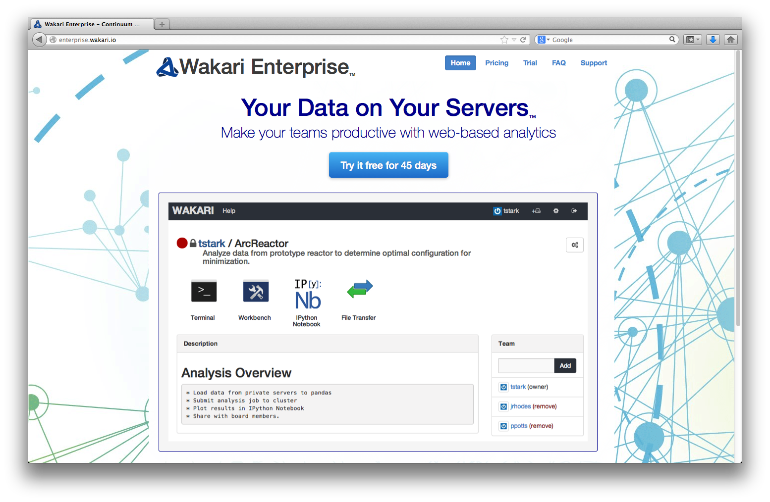
Wakari for Collaborative, Web-Based Data Analytics
Why Python for (Big) Data Analytics & Visualization?
10 years ago, Python was considered exotic in the analytics space – at best. Languages/packages like R and Matlab dominated the scene. Today, Python has become a major force in data analytics & visualization due to a number of characteristics:
- multi-purpose: prototyping, development, production, sytems administration – Python is one for all
- libraries: there is a library for almost any task or problem you face
- efficiency: Python speeds up all IT development tasks for analytics applications and reduces maintenance costs
- performance: Python has evolved from a scripting language to a 'meta' language with bridges to all high performance environments (e.g. LLVM, multi-core CPUs, GPUs, clusters)
- interoperalbility: Python seamlessly integrates with almost any other language and technology
- interactivity: Python allows domain experts to get closer to their business and financial data pools and to do real-time analytics
- collaboration: solutions like Wakari with IPython Notebook allow the easy sharing of code, data, results, graphics, etc.
![]()
The Python Quants GmbH – Python Data Exploration & Visualization
The Python Quants – the company Web site
Dr. Yves J. Hilpisch – my personal Web site
Derivatives Analytics with Python – my new book
Read an Excerpt and Order the Book
Contact Us